How we checked fasttrop • fasttrop

Key points

On four small test panels with fixed tuning parameters, the ATTs of fasttrop and of the Python package diff-diff differ by at most 4e-8.
The difference from the Python package of the authors is larger, but it is still less than 3e-5. It comes from the less accurate solver of that package.
With each change to the code, 766 test expectations run on six platforms.
With a block design and random selection of the treated units, TROP had an error 44% to 62% smaller than TWFE imputation.
In a block-design simulation that selected treated units with large trends, TROP reduced the bias, but some bias stayed.
In a staggered design with effects that differ between cohorts, a conventional TWFE regression had a bias of -0.36. TWFE imputation and TROP local had biases of -0.005 and -0.006.
With parallel trends in a staggered design, TROP local had an RMSE 4% larger than TWFE imputation.
With different trends in a staggered design, TROP local had a bias 20% smaller than TWFE imputation. But a large bias stayed.

We checked fasttrop in three ways. First, we compared its results with other implementations of TROP. Second, tests examine the tuning and the bootstrap. Third, simulations with a known effect show how well the estimates and the intervals work. They use a block design and a staggered design.

Agreement with other implementations

When two independent programs give the same numbers, an error in one of them is less likely. We compared fasttrop with two reference implementations at fixed versions:

The Python package diff-diff has the local method and the global method.
The Python package trop from the authors of the paper has the global method for a block design.

The comparison used four small test panels and five sets of fixed tuning parameters. The sets include TWFE imputation, weighted TWFE imputation, matrix completion, and two sets for the full TROP estimator. One panel has a staggered design, so it has no global estimate.

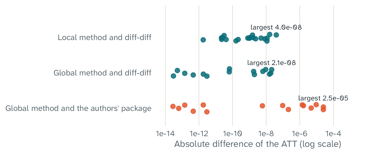
A dot chart with a log scale from 1e-14 to 1e-4. For the local and global methods compared with diff-diff, all dots are below 1e-7. For the global method compared with the package of the authors, the dots go up to 2.5e-5.

The absolute difference between the ATT of fasttrop and the ATT of each reference implementation. Each dot is one test panel with one set of tuning parameters. The axis has a log scale.

Comparison	Largest difference
Local ATT, fasttrop and `diff-diff`	4.0e-8
Local effect for each cell, fasttrop and `diff-diff`	1.1e-7
Global ATT, fasttrop and `diff-diff`	2.1e-8
Global ATT, fasttrop and the authors’ package	2.5e-5
Objective value with the same weights, relative to `diff-diff`	7e-15

A difference of 4e-8 means that the two numbers agree in the first 7 decimal places. The difference from the authors’ package is equal to the difference between the two reference implementations. The cause is the lower accuracy of the conic solver in that package. Without the low-rank term, the difference is 3e-12 or less.

The last row of the table uses the same weights in both programs. Then both programs find the same best fit, to the limit of the computer arithmetic.

Tests of the tuning and the bootstrap

The test suite examines the parts of fasttrop that the comparison above does not examine:

The leave-one-out criterion does not use a cell in its own fit or in its own unit distances.
The placebo criterion of the global method is the error of the placebo estimates.
Each bootstrap draw is equal to a new estimate on the resampled panel. fasttrop keeps the selected tuning parameters fixed in each draw. Algorithm 3 of the paper gives the resampling, but it does not say whether to select the tuning parameters again.
The weights of the local method are equal to an independent R calculation of the formula in the paper.
With lambda = c(time = 0, unit = 0, nn = Inf), the result is equal to TWFE imputation.
In a block design with no NA outcomes, TWFE imputation is equal to the result of a conventional TWFE regression. In a staggered design with effects that differ between cohorts, a test shows that the two results are different.
The number of threads does not change the results. With a seed, the results are the same in each run.

The test suite has 766 expectations. GitHub Actions runs it with R CMD check --as-cran on six platforms: Linux with four versions of R, macOS, and Windows.

Simulations with a known effect in a block design

A simulation makes many panels with a known effect. Then it measures how near the estimates are to the truth. We used three simulations with a block design. Simulations A and B have 200 panels each, and simulation A2 has 100 panels.

In each panel, the true effect is 1 for each treated cell. The untreated outcomes have unit effects, period effects, a factor with a linear trend, a second factor, and noise. All treated units start the treatment in the same period.

Simulation	Panels	Units	Treated units	Periods	Treated periods	Selection of the treated units
A	200	40	10	16	4	A random draw
A2	100	80	30	12	3	A random draw
B	200	40	10	16	4	A draw that favors the units with the largest trends

We compared three estimators:

TWFE imputation. In a block design with no NA outcomes, it gives the same estimate as a conventional TWFE regression.
The local method of TROP, with the leave-one-out criterion on 80 sampled cells.
The global method of TROP, with placebo cross-validation on 50 sets.

The tuning grid had four values for each parameter. All three estimators used the same panels. The bootstrap used 200 draws for TWFE imputation and for the global method, and 100 draws for the local method.

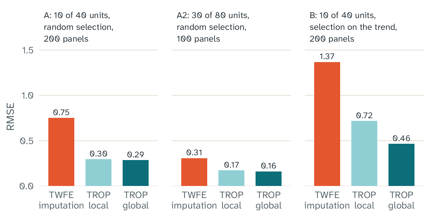
A bar chart in three panels. In simulation A, the RMSE is 0.75 for TWFE imputation, 0.30 for TROP local, and 0.29 for TROP global. In simulation A2, it is 0.31, 0.17, and 0.16. In simulation B, it is 1.37, 0.72, and 0.46.

The root mean square error (RMSE) of each estimator in each simulation. A smaller RMSE is better.

With a random selection of the treated units (simulations A and A2), all three estimators have small biases. The RMSE of TROP is 44% to 62% less than the RMSE of TWFE imputation. Thus, on average, TROP gives estimates that are nearer to the truth. In simulation A, the local method was nearer to the truth than TWFE imputation in 170 of 200 panels.

In simulation B, the selection favors the units with the largest trends. TWFE imputation has a large bias. TROP removes approximately half of this bias with the local method and two thirds with the global method, but some bias stays. The article What TROP can and cannot do explains why.

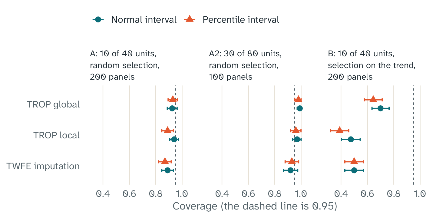
A dot chart in three panels with the normal interval and the percentile interval for each estimator. In simulations A and A2, the coverage of TROP is between 0.89 and 0.99. In simulation B, the coverage is between 0.39 and 0.70 for all estimators.

The coverage of the 95% intervals: the share of panels in which the interval contains the true effect. The dashed line is the target of 95%. The bars show two Monte Carlo standard errors.

For TROP, the coverage of the normal interval is near 95% in simulations A and A2. With 100 draws, the percentile interval of the local method has a coverage of only 89% in simulation A. For this reason, the normal interval is the default. In simulation A2, the global interval has a coverage of 99%, so it is wider than necessary. In simulation B, the bias makes the coverage of all intervals too low.

Simulations with a staggered design

In a staggered design, the treated units start the treatment in different periods. In this design, a conventional TWFE regression can give negative weights to the effects in some treated cells. Hull (2026) compares this regression with two modern estimators in 1,346 specifications from 108 papers in ten economics journals. One of the modern estimators is imputation. The study does not examine TROP.

We made three simulations with a staggered design and a known effect. Simulation C has one effect for all treated cells. Simulation D tests the problem of the regression: effects that differ between cohorts. Simulation E adds trends that differ between the cohorts.

These simulations do not repeat the study of Hull, because they use simulated data. The theory of the paper is for a block design, so they do not test the theory. They measure the bias, the error, and the coverage of the intervals.

Each panel has 60 units and 16 periods. Four cohorts of 12 units start the treatment in periods 5, 8, 11, and 14, and stay treated. The 12 other units are never treated. Thus, each panel has 360 treated cells. Each simulation has 200 panels.

Simulation	Effect in the treated cells	Trends of the untreated outcomes
C	1	Parallel
D	0.8, 0.6, 0.4, or 0.2 for the four cohorts, plus 0.1 for each period since the start	Parallel
E	The same as in D	Different between the cohorts

In simulations D and E, the effect is between 0.2 and 1.9. Its mean over the treated cells is 1. In each simulation, the truth is the mean of the effects in the treated cells.

In simulation E, the untreated outcomes also have the two factors of simulation A. The score of a unit is its loading on the linear trend plus a random number. The units with the largest scores start first. The 12 units with the smallest scores are never treated. Thus, the trends of the cohorts differ.

We compared three estimators on the same panels:

A conventional TWFE regression. It has unit effects, period effects, and one coefficient for the treatment. It uses all cells. Its standard error uses one cluster for each unit.
TWFE imputation. It fits unit effects and period effects to the untreated cells. Then it takes the mean of the estimated effects in the treated cells.
The local method of TROP. It has the same tuning grid and the same cross-validation as the simulations above.

In a block design with no NA outcomes, the regression and TWFE imputation give the same estimate. In a staggered design, they can differ. The regression gives its own weights to the treated cells. The two other estimators give the weight 1 to each treated cell.

The global method is only for a block design, so we did not use it. The bootstrap had 200 draws for TWFE imputation and 100 draws for the local method. It kept the tuning parameters fixed. The regression has a normal interval only.

The weights of the regression

With parallel trends, the regression estimates a weighted mean of the effects in the treated cells. The weights depend only on the start periods of the cohorts.

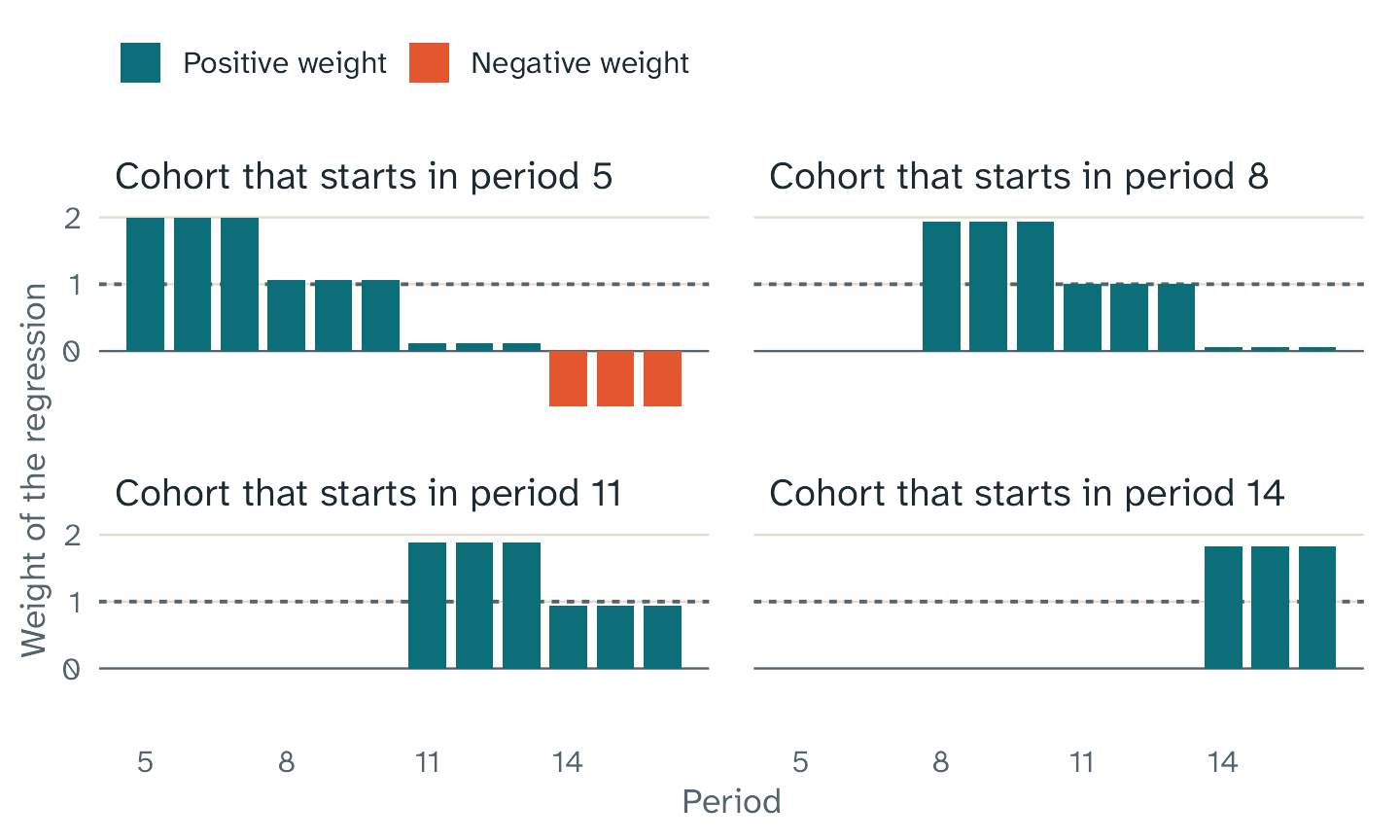
A bar chart in four panels, one for each cohort. For the cohort that starts in period 5, the weight is 2.0 in the first three periods and -0.82 in the last three periods. For the other cohorts, the weights are between 0.06 and 1.94. The dashed line is the weight 1 of TWFE imputation.

The weight of the regression on the treated cells. Each bar is one cohort in one period. The dashed line is the weight 1 of TWFE imputation. The mean weight is 1.

In 3 of the 30 groups, the weight is negative. These are the periods 14 to 16 of the cohort that starts in period 5. In simulations D and E, these cells have the largest effects of the design. With these weights, the weighted mean of the effects is 0.64, and the true mean is 1.

The results

The table has the results. The bias has its Monte Carlo standard error in parentheses. The column “SD” is the standard deviation of the estimates over the panels, and “Mean SE” is the mean of the standard errors. The last two columns are the coverage of the 95% intervals.

Simulation	Estimator	Bias (MC SE)	SD	Mean SE	RMSE	Normal interval	Percentile interval
C	TWFE regression	-0.005 (0.004)	0.055	0.056	0.055	95.5%	None
	TWFE imputation	-0.005 (0.004)	0.063	0.063	0.063	97.5%	95.0%
	TROP local	-0.006 (0.005)	0.066	0.065	0.066	97.0%	95.5%
D	TWFE regression	-0.361 (0.004)	0.055	0.067	0.366	0.0%	None
	TWFE imputation	-0.005 (0.004)	0.063	0.080	0.063	98.5%	98.5%
	TROP local	-0.006 (0.005)	0.066	0.082	0.066	98.0%	96.0%
E	TWFE regression	0.225 (0.011)	0.162	0.209	0.277	91.5%	None
	TWFE imputation	1.257 (0.017)	0.238	0.250	1.280	0.0%	0.5%
	TROP local	1.006 (0.015)	0.215	0.214	1.029	0.5%	0.5%

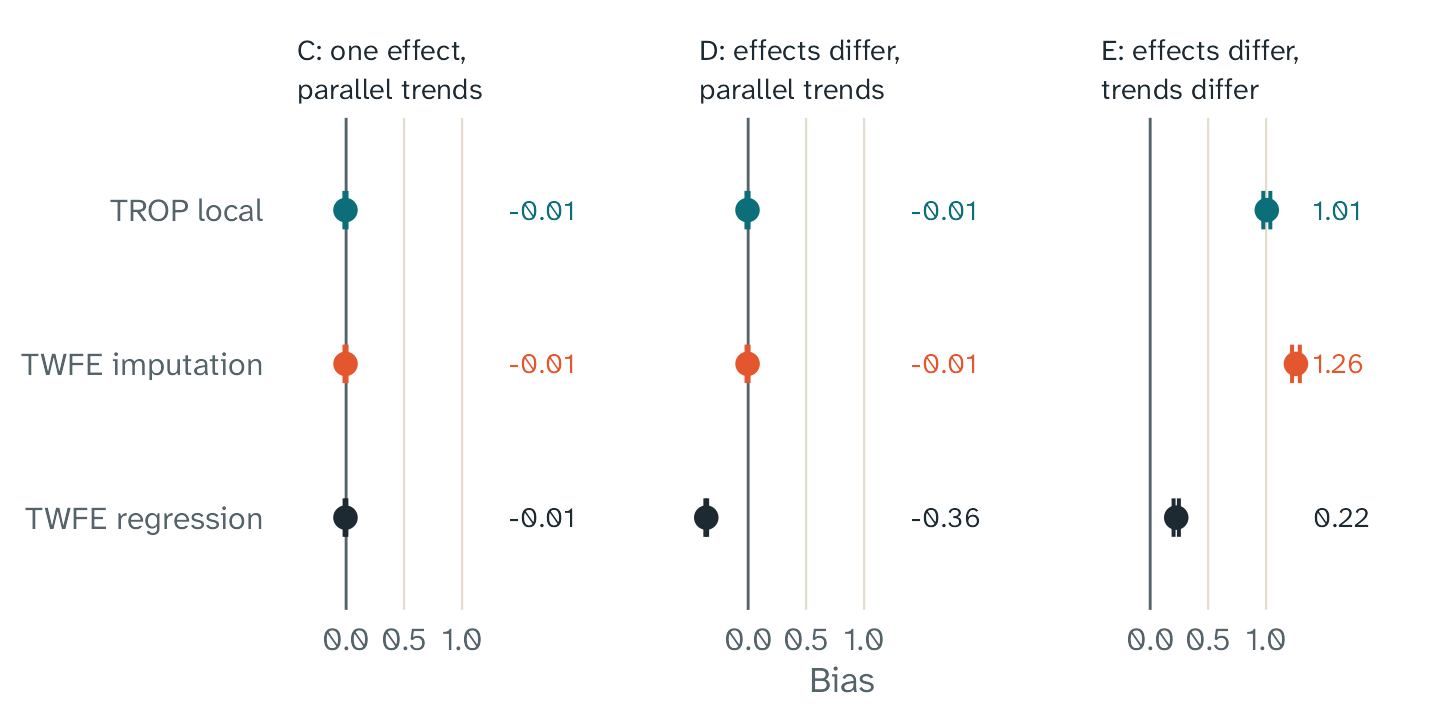
A dot chart in three panels, one for each simulation. It shows the bias of each estimator. In simulation C, it is -0.01 for TWFE regression, -0.01 for TWFE imputation, and -0.01 for TROP local. In simulation D, it is -0.36 for TWFE regression, -0.01 for TWFE imputation, and -0.01 for TROP local. In simulation E, it is 0.22 for TWFE regression, 1.26 for TWFE imputation, and 1.01 for TROP local.

The bias of each estimator. The number at the right of each row is the bias. The true effect is the mean of the effects in the treated cells. The bars show two Monte Carlo standard errors.

In simulation C, the three estimators have small biases. Each bias is less than two Monte Carlo standard errors from zero. The regression has the smallest standard deviation. Its model is correct in simulation C, and it uses the treated cells in the fit.

In simulation D, the bias of the regression is -0.36. Thus, its mean estimate is 63.9% of the true effect. Its 95% interval contains the truth in 0 of the 200 panels. TWFE imputation and the local method have the same biases as in simulation C. They use only the untreated cells in the fit, and the panels have the same noise in both simulations.

In simulation E, the biases of TWFE imputation and of the local method are large. They are 1.26 and 1.01, and the true effect is 1. The local method has a bias 20% smaller and an RMSE 20% smaller than TWFE imputation. But the mean estimate of the local method is 2.0 times the true effect.

In simulation E, the regression has the smallest bias, 0.22. This result does not show an advantage of the regression. Its bias has two parts. The weights give -0.36, as in simulation D. The different trends add approximately 0.58. The two parts have opposite signs, so they partly cancel, but in another design they can have the same sign.

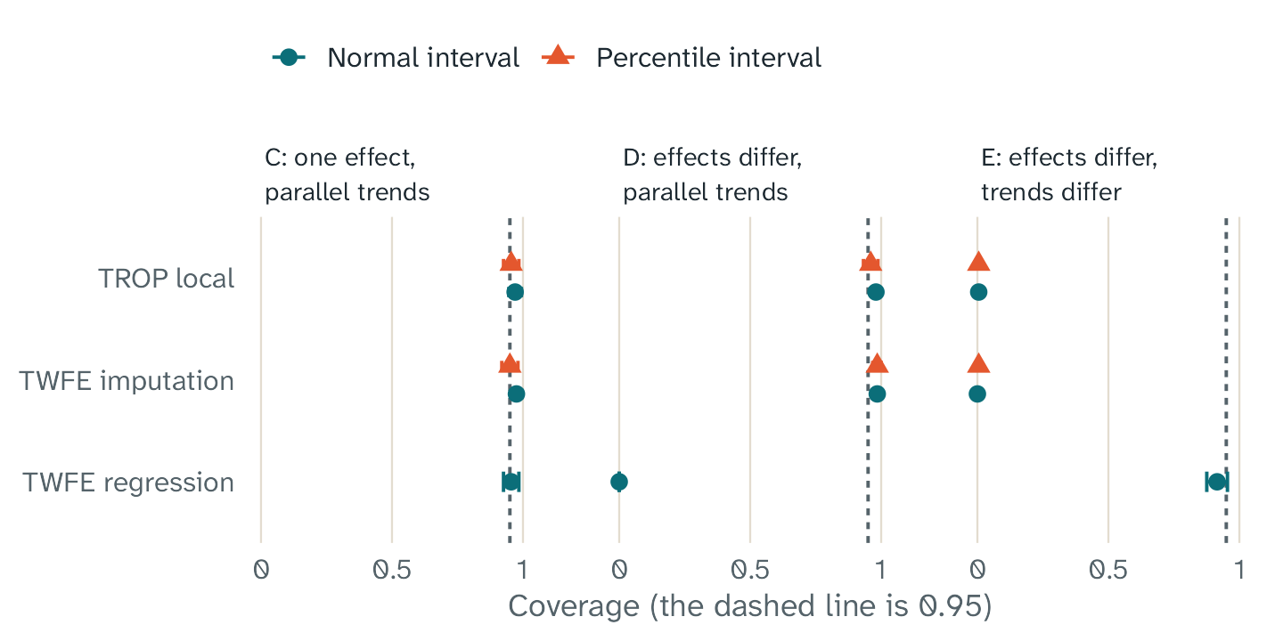
A dot chart in three panels, one for each simulation. It shows the coverage of the 95% normal interval of each estimator. The target is 95%. In simulation C, it is 95.5% for TWFE regression, 97.5% for TWFE imputation, and 97.0% for TROP local. In simulation D, it is 0.0% for TWFE regression, 98.5% for TWFE imputation, and 98.0% for TROP local. In simulation E, it is 91.5% for TWFE regression, 0.0% for TWFE imputation, and 0.5% for TROP local.

The coverage of the 95% intervals: the share of panels in which the interval contains the true effect. The dashed line is the target of 95%. The bars show two Monte Carlo standard errors.

In simulation D, the intervals of TWFE imputation and of the local method are wider than necessary. The mean standard error of TWFE imputation is 0.080, but the standard deviation of its estimates is 0.063. The coverage of its normal interval is 98.5%, and the coverage of its percentile interval is 98.5%. The local method has the same pattern.

We think that the bootstrap causes this result. It resamples the treated units, so the number of units in each cohort changes in each draw. The effect differs between the cohorts, so the mean effect also changes. Each simulated panel has 12 units in each cohort. We did not test this cause in a saved simulation.

In simulation E, the intervals of TWFE imputation and of the local method contain the true effect in at most 1 of the 200 panels. The bias is large compared with the standard deviation of the estimates, which is 0.24 and 0.21. The normal interval of the regression has a coverage of 91.5%.

These simulations have limits. They use one design with 60 units, 16 periods, and four cohorts. They also use one tuning grid. The noise is independent between the cells, but the noise in real panels can have correlation over time.

We did not test the other modern estimator of Hull. It averages the DiD estimates of each cohort and period. We also did not compare TROP with a modern estimator on real data. Hull recommends this comparison for each application.

Covariates

The article Use covariates gives the checks of the covariates. In summary:

On three test panels, fasttrop and an independent solution of Eq. 13 with covariates agree to 6.7e-09 or better.
In a simulation with a covariate bias after the treatment starts, the bias of TROP local decreased from 1.45 to 0.01 with covariates.

The scripts and the data

The package contains the scripts and the results, so you can run the checks again. We ran the simulation scripts and the comparison scripts only on Windows. GitHub Actions runs the test suite on Linux, macOS, and Windows.

The folder inst/validation of the source package has the simulation scripts and the comparison report. In an installed package, use system.file("validation", package = "fasttrop") to find it.
The folder tests/testthat has the test suite and the reference results.
The script data-raw/oracle_fixtures.py in the GitHub repository made the reference results.