Choosing Employment Weights: OEWS versus PUMS

Weights answer a population question. OEWS is usually the best choice when the target is official occupation employment and wage context. PUMS is useful when the target is a custom sample or demographic cell.

Start with the Same O*NET Score

abilities <- onet_archive_read(
  "30.3",
  "Abilities",
  path = archive_303,
  release_date = "2026-05-01"
)

score <- abilities |>
  filter(element_id == "1.A.1.a.1") |>
  transmute(onet_soc_code, measure_score = data_value)

score |>
  onet_kable()

onet_soc_code	measure_score
15-1252.00	4.35
29-1141.00	4.71
11-1011.00	4.50
41-1011.00	4.15

OEWS Weights

oews_weights <- onet_weight_panel_oews(
  onet_oews_national(2024, path = oews_path),
  year = 2024
)

oews_result <- onet_measure_aggregate(
  score,
  oews_weights,
  measure_id = "oral_comprehension_fixture"
)

oews_weights |>
  onet_kable()

reference_soc_code	year	employment	weight_share	source	source_taxonomy	reference_taxonomy
11-1011	2024	211230	0.040	OEWS	2018 SOC	2018 SOC
15-1252	2024	1847900	0.353	OEWS	2018 SOC	2018 SOC
29-1141	2024	3175400	0.607	OEWS	2018 SOC	2018 SOC

oews_result |>
  select(-coverage, -provenance) |>
  onet_kable()

measure_id	aggregate	total_employment	covered_employment	employment_coverage_share	n_occupations	n_reference_soc
oral_comprehension_fixture	4.574	5234530	5234530	1	4	4

PUMS Weights

pums <- tibble::tibble(
  SOCP = c("151252", "151252", "291141", "291141", "111011", "111011"),
  PWGTP = c(120, 80, 90, 110, 10, 30),
  sex = c("F", "M", "F", "M", "F", "M")
)

pums_weights <- onet_weight_panel_pums(
  pums,
  year = 2022,
  group = "sex"
)

pums_f <- onet_measure_aggregate(
  score,
  pums_weights,
  measure_id = "oral_comprehension_fixture",
  cell = list(sex = "F")
)
pums_m <- onet_measure_aggregate(
  score,
  pums_weights,
  measure_id = "oral_comprehension_fixture",
  cell = list(sex = "M")
)

pums_weights |>
  onet_kable()

reference_soc_code	sex	year	employment	weight_share	source	source_taxonomy	reference_taxonomy
11-1011	F	2022	10	0.023	PUMS	2018 SOC	2018 SOC
11-1011	M	2022	30	0.068	PUMS	2018 SOC	2018 SOC
15-1252	F	2022	120	0.273	PUMS	2018 SOC	2018 SOC
15-1252	M	2022	80	0.182	PUMS	2018 SOC	2018 SOC
29-1141	F	2022	90	0.205	PUMS	2018 SOC	2018 SOC
29-1141	M	2022	110	0.250	PUMS	2018 SOC	2018 SOC

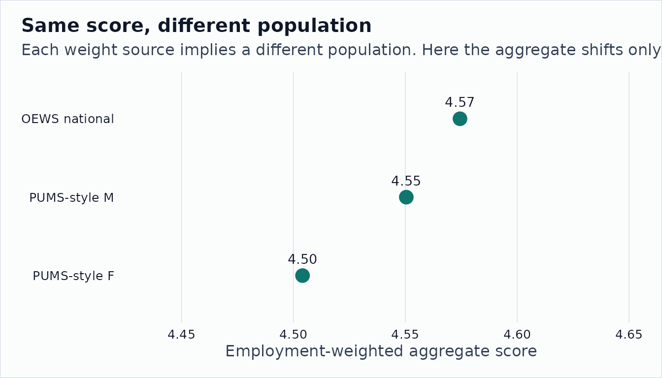
Compare the Answers

comparison <- tibble::tibble(
  population = c("OEWS national", "PUMS-style F", "PUMS-style M"),
  aggregate = c(oews_result$aggregate, pums_f$aggregate, pums_m$aggregate),
  coverage = c(
    oews_result$employment_coverage_share,
    pums_f$employment_coverage_share,
    pums_m$employment_coverage_share
  )
)

comparison |>
  onet_kable()

population	aggregate	coverage
OEWS national	4.574	1
PUMS-style F	4.504	1
PUMS-style M	4.550	1

score_span <- range(comparison$aggregate)
pad <- max(0.05, diff(score_span))

ggplot2::ggplot(comparison, ggplot2::aes(
  x = aggregate,
  y = stats::reorder(population, aggregate)
)) +
  ggplot2::geom_point(color = onet2r_colors[["teal"]], size = 4.5) +
  ggplot2::geom_text(
    ggplot2::aes(label = sprintf("%.2f", aggregate)),
    vjust = -1.2,
    size = 3.6,
    color = onet2r_colors[["ink"]]
  ) +
  ggplot2::coord_cartesian(
    xlim = c(score_span[1] - pad, score_span[2] + pad)
  ) +
  ggplot2::labs(
    title = "Same score, different population",
    subtitle = paste(
      "Each weight source implies a different population.",
      "Here the aggregate shifts only slightly."
    ),
    x = "Employment-weighted aggregate score",
    y = NULL
  ) +
  onet2r_theme()

If your claim is about the national labor market, OEWS is the natural default. If your claim is about a subgroup, geography, or survey-defined population, build a PUMS weight panel and state the cell explicitly.