How to Fool Yourself with O*NET over Time

A common mistake is to treat every release-to-release difference as a fresh within-occupation change. O*NET archives contain source dates, domain sources, suppression flags, and taxonomy vintages. Ignoring those fields can turn a carryforward, transition row, or crosswalk seam into a misleading trend.

Do not start with the coefficient. Start with the audit fields. If a result depends on rows that were carried forward, bridged across a split, or marked as transition data, the caveat belongs next to the estimate.

The Naive Difference

panel <- onet_panel(
  "Abilities",
  versions = c("30.2", "30.3"),
  scale = "IM",
  archives = c(
    `30.2` = file.path(archive_base, "db_30_2_text"),
    `30.3` = file.path(archive_base, "db_30_3_text")
  ),
  release_dates = c(`30.2` = "2026-02-01", `30.3` = "2026-05-01")
)

naive <- panel |>
  select(release_version, onet_soc_code, element_id, element_name, data_value)

naive <- naive |>
  filter(release_version == "30.2") |>
  select(onet_soc_code, element_id, element_name, from_value = data_value) |>
  inner_join(
    naive |>
      filter(release_version == "30.3") |>
      select(onet_soc_code, element_id, to_value = data_value),
    by = join_by(onet_soc_code, element_id),
    relationship = "one-to-one"
  ) |>
  mutate(naive_change = to_value - from_value) |>
  arrange(desc(abs(naive_change)))

naive |>
  head(8) |>
  onet_kable()

onet_soc_code	element_id	element_name	from_value	to_value	naive_change
29-1141.00	1.A.1.b.1	Problem Sensitivity	4.60	4.90	0.30
15-1252.00	1.A.1.a.1	Oral Comprehension	4.12	4.35	0.23
41-1011.00	1.A.1.a.1	Oral Comprehension	4.00	4.15	0.15
11-1011.00	1.A.1.a.1	Oral Comprehension	4.38	4.50	0.12
15-1252.00	1.A.1.b.1	Problem Sensitivity	4.50	4.50	0.00
29-1141.00	1.A.1.a.1	Oral Comprehension	4.71	4.71	0.00
11-1011.00	1.A.1.b.1	Problem Sensitivity	4.22	4.22	0.00

The naive table is useful as a screening tool. It is not enough for an interpretation.

The Reconciled Difference

changes <- onet_panel_reconcile(panel, onet_crosswalk_bridge("2019", "2019"))

changes |>
  select(
    to_soc_code,
    element_name,
    value_change,
    change_type,
    from_source_date,
    to_source_date,
    method_break,
    safely_comparable
  ) |>
  arrange(desc(abs(value_change))) |>
  head(8) |>
  onet_kable()

to_soc_code	element_name	value_change	change_type	from_source_date	to_source_date	method_break	safely_comparable
29-1141	Problem Sensitivity	0.30	recode_or_recalc_flag	2024-08-01	2024-08-01	FALSE	FALSE
15-1252	Oral Comprehension	0.23	real_update	2024-07-01	2025-07-01	FALSE	TRUE
41-1011	Oral Comprehension	0.15	real_update	2024-06-01	2025-06-01	FALSE	TRUE
11-1011	Oral Comprehension	0.12	real_update	2024-07-01	2025-07-01	TRUE	FALSE
15-1252	Problem Sensitivity	0.00	stale_carryforward	2024-07-01	2024-07-01	FALSE	TRUE
29-1141	Oral Comprehension	0.00	resampled_stable	2024-08-01	2025-08-01	FALSE	TRUE
11-1011	Problem Sensitivity	0.00	stale_carryforward	2024-07-01	2024-07-01	FALSE	TRUE

Now the same differences have labels. A change without a source-date change is not as strong as a change with fresh source data. A method break should be treated as a warning rather than as clean within-occupation change.

A useful rule of thumb. Use value_change to find rows worth inspecting, then use change_type, method_break, and safely_comparable to decide what those rows can support.

The Taxonomy Seam

cross_panel <- onet_panel(
  "Abilities",
  versions = c("24.3", "25.1"),
  scale = "IM",
  archives = c(
    `24.3` = file.path(archive_base, "db_24_3_text"),
    `25.1` = file.path(archive_base, "db_25_1_text")
  ),
  release_dates = c(`24.3` = "2020-08-01", `25.1` = "2020-11-01")
)

bridge <- tibble::tibble(
  from_vintage = "2010",
  to_vintage = "2019",
  from_onet_soc_code = c("15-1132.00", "15-1132.00", "29-1141.00"),
  to_onet_soc_code = c("15-1252.00", "15-1253.00", "29-1141.00"),
  map_type = c("split", "split", "one_to_one"),
  crosswalk_weight = c(0.5, 0.5, 1)
)

seam <- onet_panel_reconcile(cross_panel, bridge)

seam |>
  select(
    from_onet_soc_code,
    to_onet_soc_code,
    element_name,
    change_type,
    transition_data,
    crosswalk_uncertain,
    safely_comparable
  ) |>
  onet_kable()

from_onet_soc_code	to_onet_soc_code	element_name	change_type	transition_data	crosswalk_uncertain	safely_comparable
15-1132.00	15-1252.00	Oral Comprehension	transition_data	TRUE	TRUE	FALSE
15-1132.00	15-1253.00	Oral Comprehension	transition_data	TRUE	TRUE	FALSE
29-1141.00	29-1141.00	Oral Comprehension	real_update	FALSE	FALSE	TRUE
15-1132.00	15-1252.00	Problem Sensitivity	dropped	FALSE	TRUE	FALSE
15-1132.00	15-1253.00	Problem Sensitivity	dropped	FALSE	TRUE	FALSE

safe_counts <- seam |>
  mutate(comparability = if_else(safely_comparable, "Safe", "Not safe")) |>
  count(comparability, name = "rows")

ggplot2::ggplot(safe_counts, ggplot2::aes(
  x = comparability,
  y = rows,
  fill = comparability
)) +
  ggplot2::geom_col(width = 0.6, show.legend = FALSE) +
  ggplot2::coord_flip() +
  ggplot2::scale_fill_manual(
    values = c("Safe" = onet2r_colors[["teal"]], "Not safe" = onet2r_colors[["rose"]])
  ) +
  ggplot2::labs(
    title = "Taxonomy Seams Reduce Safe Comparisons",
    subtitle = "A split occupation carries extra uncertainty even when codes can be bridged.",
    x = NULL,
    y = "Rows"
  ) +
  onet2r_theme()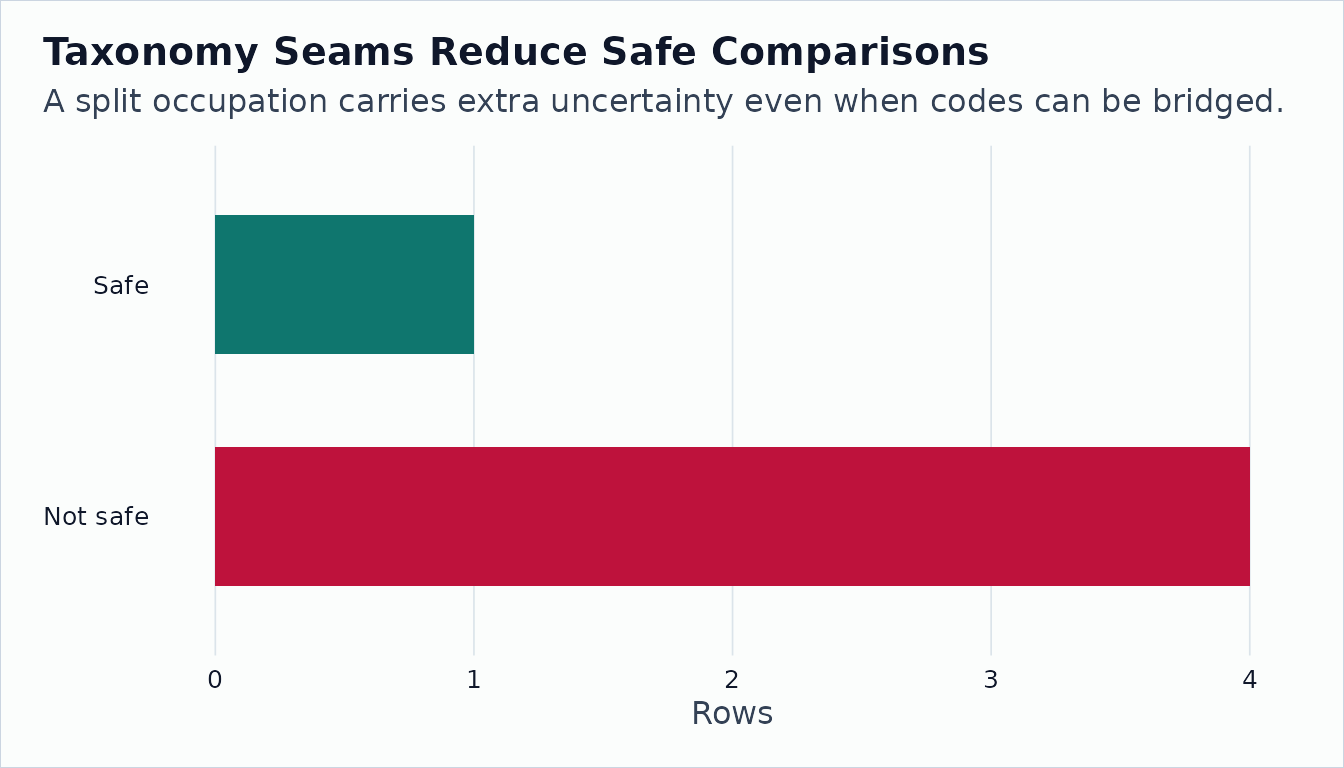

Before making a historical claim, ask: Did the value change? Did the source date change? Did the occupation cross a taxonomy seam? Was either row transition data or suppressed? The package gives you those fields so the caveats do not get lost.