Within-Versus-Between Decomposition

Aggregate changes can come from two places. Occupations can change internally, or employment can shift toward occupations that already had different scores. With O*NET, the within term needs an extra gate: only rows that survive the comparability checks should be counted as safely comparable within-occupation change.

A Fixture-Derived Example

archive_base <- system.file("extdata", "onet-mini", package = "onet2r")
cross_panel <- onet_panel(
  "Abilities",
  versions = c("24.3", "25.1"),
  scale = "IM",
  archives = c(
    `24.3` = file.path(archive_base, "db_24_3_text"),
    `25.1` = file.path(archive_base, "db_25_1_text")
  ),
  release_dates = c(`24.3` = "2020-08-01", `25.1` = "2020-11-01")
)

bridge <- tibble::tibble(
  from_vintage = "2010",
  to_vintage = "2019",
  from_onet_soc_code = c("15-1132.00", "15-1132.00", "29-1141.00"),
  to_onet_soc_code = c("15-1252.00", "15-1253.00", "29-1141.00"),
  map_type = c("split", "split", "one_to_one"),
  crosswalk_weight = c(0.5, 0.5, 1)
)

ability_changes <- onet_panel_reconcile(cross_panel, bridge)
score_changes <- ability_changes |>
  filter(element_id == "1.A.1.a.1", !is.na(from_value), !is.na(to_value)) |>
  mutate(reference_soc_code = sub("\\.\\d{2}$", "", to_onet_soc_code))

from_scores <- score_changes |>
  select(
    reference_soc_code,
    measure_score = from_value,
    safely_comparable
  )
to_scores <- score_changes |>
  select(
    reference_soc_code,
    measure_score = to_value,
    safely_comparable
  )

from_weights <- tibble::tibble(
  reference_soc_code = c("15-1252", "15-1253", "29-1141"),
  employment = c(120, 80, 200)
)
to_weights <- tibble::tibble(
  reference_soc_code = c("15-1252", "15-1253", "29-1141"),
  employment = c(170, 110, 160)
)

from_scores |>
  onet_kable()

reference_soc_code	measure_score	safely_comparable
15-1252	4.2	FALSE
15-1253	4.2	FALSE
29-1141	4.6	TRUE

to_scores |>
  onet_kable()

reference_soc_code	measure_score	safely_comparable
15-1252	4.48	FALSE
15-1253	4.30	FALSE
29-1141	4.66	TRUE

The comparability flag comes from onet_panel_reconcile(), not from a hand-labeled example table. Rows that cross the split with transition data are kept in the accounting but do not get treated as clean within-occupation change.

decomp <- onet_decompose_change(
  from_scores,
  to_scores,
  from_weights,
  to_weights
)

decomp |>
  select(component, value) |>
  onet_kable()

component	value
within	0.030
between	-0.055
interaction	0.021
unclassifiable	0.104
total_change	0.100

onet_coverage(decomp) |>
  onet_kable()

n_common	n_safely_comparable	leakage
3	1	0

components <- decomp |>
  filter(component != "total_change") |>
  mutate(
    label = tools::toTitleCase(gsub("_", " ", component)),
    label = factor(label, levels = rev(label)),
    direction = if_else(value >= 0, "Raises the aggregate", "Lowers the aggregate")
  )

ggplot2::ggplot(components, ggplot2::aes(x = value, y = label, fill = direction)) +
  ggplot2::geom_col(width = 0.62) +
  ggplot2::geom_vline(xintercept = 0, color = onet2r_colors[["slate"]]) +
  ggplot2::geom_text(
    ggplot2::aes(
      label = sprintf("%+.3f", value),
      hjust = if_else(value >= 0, -0.15, 1.15)
    ),
    size = 3.5,
    color = onet2r_colors[["ink"]]
  ) +
  ggplot2::scale_fill_manual(
    values = c(
      "Raises the aggregate" = onet2r_colors[["teal"]],
      "Lowers the aggregate" = onet2r_colors[["rose"]]
    )
  ) +
  ggplot2::scale_x_continuous(
    expand = ggplot2::expansion(mult = c(0.16, 0.16))
  ) +
  ggplot2::labs(
    title = "Where did the aggregate change come from?",
    subtitle = "Each piece's contribution to the total change.",
    x = "Contribution to total change",
    y = NULL,
    fill = NULL
  ) +
  onet2r_theme()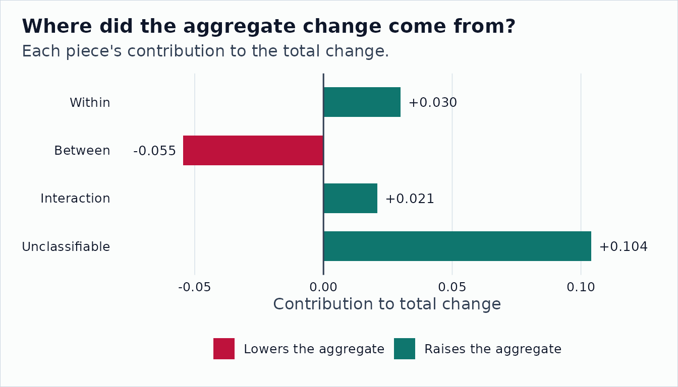

The component rows other than total_change sum to the total change.

decomp |>
  summarise(
    component_sum = sum(value[component != "total_change"]),
    total_change = value[component == "total_change"],
    difference = component_sum - total_change
  ) |>
  onet_kable()

component_sum	total_change	difference
0.1	0.1	0

A Demographic Split

The same decomposition can be run after users prepare weight panels for demographic cells. The package does not download raw PUMS data in examples, but the fixture below follows the same reference-SOC, cell, employment shape.

from_weights_by_sex <- tibble::tibble(
  reference_soc_code = c("15-1252", "29-1141", "15-1252", "29-1141"),
  sex = c("F", "F", "M", "M"),
  employment = c(40, 70, 60, 30)
)
to_weights_by_sex <- tibble::tibble(
  reference_soc_code = c("15-1252", "29-1141", "15-1252", "29-1141"),
  sex = c("F", "F", "M", "M"),
  employment = c(70, 50, 80, 0)
)

split_results <- lapply(unique(from_weights_by_sex$sex), function(cell) {
  result <- onet_decompose_change(
    from_scores,
    to_scores,
    from_weights_by_sex |> filter(sex == cell),
    to_weights_by_sex |> filter(sex == cell)
  )
  result$sex <- cell
  result
}) |>
  purrr::list_rbind()

split_results |>
  select(sex, component, value) |>
  onet_kable()

sex	component	value
F	within	0.038
F	between	-0.088
F	interaction	0.048
F	unclassifiable	0.102
F	total_change	0.100
M	within	0.020
M	between	-0.133
M	interaction	0.073
M	unclassifiable	0.187
M	total_change	0.147

Each cell has its own weight shift and its own unclassifiable bucket. That is the part reviewers need to see when an aggregate result depends on vintage bridges, source dates, or task-handling choices.