Adding OEWS Wage and Employment Context

O*NET tells you what occupations do: their tasks, abilities, skills, knowledge, and work contexts. The Bureau of Labor Statistics Occupational Employment and Wage Statistics (OEWS) program tells you how large those occupations are in the labor market and what they pay. Joining the two lets you move from an occupation-level descriptor table to a labor-market-weighted question.

This walkthrough asks: among occupations in a small O*NET ability panel, what does a national employment-weighted ability score look like, and what changes if we use a custom PUMS-style population instead?

Read OEWS Estimates

onet_oews_national() normalizes BLS OEWS files into snake_case columns and parses formatted employment and wage fields into numeric values.

oews <- onet_oews_national(year = 2024, path = sample_oews)

oews |>
  select(occ_code, occ_title, tot_emp, a_median, h_median) |>
  onet_kable()

occ_code	occ_title	tot_emp	a_median	h_median
15-1252	Software Developers	1847900	133080	63.98
29-1141	Registered Nurses	3175400	93070	44.75
11-1011	Chief Executives	211230	206680	99.37

Build a Reference-SOC Weight Panel

OEWS uses 6-digit SOC codes. O*NET archive tables use 8-digit O*NET-SOC detail codes. The weight-panel helper records the source and reference taxonomy so the join is auditable.

oews_weights <- onet_weight_panel_oews(oews, year = 2024)

oews_weights |>
  onet_kable()

reference_soc_code	year	employment	weight_share	source	source_taxonomy	reference_taxonomy
11-1011	2024	211230	0.040	OEWS	2018 SOC	2018 SOC
15-1252	2024	1847900	0.353	OEWS	2018 SOC	2018 SOC
29-1141	2024	3175400	0.607	OEWS	2018 SOC	2018 SOC

Get O*NET Occupation Scores from an Archive

The occupation scores below come from onet_archive_read(), not a hand-built example table. We use Oral Comprehension as a concrete descriptor because it is available in the bundled fixture.

abilities <- onet_archive_read(
  "30.3",
  "Abilities",
  path = archive_303,
  release_date = "2026-05-01"
)

oral_scores <- abilities |>
  filter(element_id == "1.A.1.a.1") |>
  transmute(
    onet_soc_code,
    title,
    measure_score = data_value
  )

oral_scores |>
  onet_kable()

onet_soc_code	title	measure_score
15-1252.00	Software Developers	4.35
29-1141.00	Registered Nurses	4.71
11-1011.00	Chief Executives	4.50
41-1011.00	First-Line Supervisors of Retail Sales Workers	4.15

Aggregate with OEWS Employment

oral_oews <- onet_measure_aggregate(
  oral_scores,
  oews_weights,
  measure_id = "oral_comprehension_fixture"
)

oral_oews |>
  select(-coverage, -provenance) |>
  onet_kable()

measure_id	aggregate	total_employment	covered_employment	employment_coverage_share	n_occupations	n_reference_soc
oral_comprehension_fixture	4.574	5234530	5234530	1	4	4

onet_provenance(oral_oews) |>
  onet_kable()

measure_id	weight_source	weight_year	source_taxonomy	reference_taxonomy	bridge_used	crosswalk_path
oral_comprehension_fixture	OEWS	2024	2018 SOC	2018 SOC	FALSE	2018 SOC -> 2018 SOC

The aggregate is the employment-weighted score for occupations covered by both the O*NET fixture and the OEWS sample. Coverage tells you how much of the weight panel was included.

onet_coverage(oral_oews) |>
  onet_kable()

measure_id	total_employment	covered_employment	employment_coverage_share	n_occupations	n_reference_soc
oral_comprehension_fixture	5234530	5234530	1	4	4

Inspect Occupation Contributions

contributions <- oral_scores |>
  mutate(reference_soc_code = sub("\\.\\d{2}$", "", onet_soc_code)) |>
  inner_join(oews_weights, by = join_by(reference_soc_code), relationship = "many-to-one") |>
  mutate(weighted_score = measure_score * employment) |>
  arrange(desc(weighted_score)) |>
  select(title, reference_soc_code, measure_score, employment, weight_share, weighted_score)

contributions |>
  onet_kable()

title	reference_soc_code	measure_score	employment	weight_share	weighted_score
Registered Nurses	29-1141	4.71	3175400	0.607	14956134
Software Developers	15-1252	4.35	1847900	0.353	8038365
Chief Executives	11-1011	4.50	211230	0.040	950535

ggplot2::ggplot(contributions, ggplot2::aes(
  x = weighted_score,
  y = stats::reorder(title, weighted_score)
)) +
  ggplot2::geom_col(fill = onet2r_colors[["teal"]], width = 0.65) +
  ggplot2::scale_x_continuous(
    labels = scales::label_number(scale_cut = scales::cut_short_scale()),
    expand = ggplot2::expansion(mult = c(0, 0.05))
  ) +
  ggplot2::labs(
    title = "Which Occupations Drive the Weighted Score?",
    subtitle = "Contribution is the occupation score times employment.",
    x = "Score times employment",
    y = NULL
  ) +
  onet2r_theme()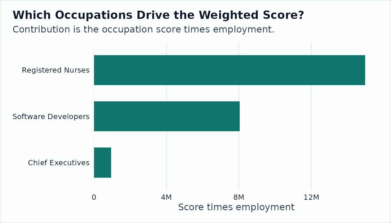

Compare OEWS with a PUMS-Style Weight Panel

OEWS is the right default for official occupation employment and wage context. PUMS-derived weights are useful when the target population is a custom sample, geography, or demographic cell.

pums <- tibble::tibble(
  SOCP = c("151252", "151252", "291141", "291141", "111011"),
  PWGTP = c(120, 80, 90, 110, 20),
  sex = c("F", "M", "F", "M", "F")
)

pums_weights <- onet_weight_panel_pums(
  pums,
  year = 2022,
  group = "sex"
)

pums_weights |>
  onet_kable()

reference_soc_code	sex	year	employment	weight_share	source	source_taxonomy	reference_taxonomy
11-1011	F	2022	20	0.048	PUMS	2018 SOC	2018 SOC
15-1252	F	2022	120	0.286	PUMS	2018 SOC	2018 SOC
15-1252	M	2022	80	0.190	PUMS	2018 SOC	2018 SOC
29-1141	F	2022	90	0.214	PUMS	2018 SOC	2018 SOC
29-1141	M	2022	110	0.262	PUMS	2018 SOC	2018 SOC

Because this PUMS-style panel has cells, pick one cell before aggregating.

oral_pums_f <- onet_measure_aggregate(
  oral_scores,
  pums_weights,
  measure_id = "oral_comprehension_fixture",
  cell = list(sex = "F")
)

tibble::tibble(
  weight_source = c("OEWS national", "PUMS-style F cell"),
  aggregate = c(oral_oews$aggregate, oral_pums_f$aggregate),
  coverage = c(
    oral_oews$employment_coverage_share,
    oral_pums_f$employment_coverage_share
  )
) |>
  onet_kable()

weight_source	aggregate	coverage
OEWS national	4.574	1
PUMS-style F cell	4.504	1

Neither source is always better. OEWS gives official labor market estimates; PUMS gives custom cells. The package records the weight source, year, taxonomy, and coverage so a reader can see what changed.