Stress-Testing a User-Supplied Exposure Measure

This article uses a stylized task score to show the sensitivity workflow. The score is not a package-endorsed exposure measure. The package’s job is to show how much the headline number moves when non-substantive choices change.

Build the Measure from Task Files

tasks_243 <- onet_archive_read(
  "24.3",
  "Task Statements",
  path = archive_path("24.3"),
  release_date = "2020-08-01"
)
ratings_243 <- onet_archive_read(
  "24.3",
  "Task Ratings",
  path = archive_path("24.3"),
  release_date = "2020-08-01"
)
tasks_251 <- onet_archive_read(
  "25.1",
  "Task Statements",
  path = archive_path("25.1"),
  release_date = "2020-11-01"
)
ratings_251 <- onet_archive_read(
  "25.1",
  "Task Ratings",
  path = archive_path("25.1"),
  release_date = "2020-11-01"
)

task_scores <- tibble::tibble(
  task_id = c("1101", "1201", "1202", "2101"),
  score = c(0.75, 0.80, 0.55, 0.25)
)

measure <- onet_measure(
  task_scores,
  key = "task_id",
  score = "score",
  key_type = "task",
  universe = unique(c(tasks_243$task_id, tasks_251$task_id)),
  measure_id = "stylized_exposure",
  release_version = "multi_release_fixture"
)

onet_coverage(measure) |>
  onet_kable()

key_type	n_input	n_universe	n_matched	coverage_share	employment_coverage_share
task	4	4	4	1	NA

Create Alternative Weight Panels

oews_weights <- onet_weight_panel_oews(
  onet_oews_national(2024, path = oews_path),
  year = 2024
)

pums <- tibble::tibble(
  SOCP = c("151252", "151253", "291141", "291141"),
  PWGTP = c(80, 120, 200, 80)
)
pums_weights <- onet_weight_panel_pums(pums, year = 2022)

oews_weights |>
  onet_kable()

reference_soc_code	year	employment	weight_share	source	source_taxonomy	reference_taxonomy
11-1011	2024	211230	0.040	OEWS	2018 SOC	2018 SOC
15-1252	2024	1847900	0.353	OEWS	2018 SOC	2018 SOC
29-1141	2024	3175400	0.607	OEWS	2018 SOC	2018 SOC

pums_weights |>
  onet_kable()

reference_soc_code	year	employment	weight_share	source	source_taxonomy	reference_taxonomy
15-1252	2022	80	0.167	PUMS	2018 SOC	2018 SOC
15-1253	2022	120	0.250	PUMS	2018 SOC	2018 SOC
29-1141	2022	280	0.583	PUMS	2018 SOC	2018 SOC

Run the Sensitivity Grid

bridge_2010_2019 <- tibble::tibble(
  from_vintage = "mixed_fixture",
  to_vintage = "2018 SOC",
  from_onet_soc_code = c(
    "15-1132.00",
    "15-1132.00",
    "15-1252.00",
    "15-1253.00",
    "29-1141.00"
  ),
  to_onet_soc_code = c(
    "15-1252.00",
    "15-1253.00",
    "15-1252.00",
    "15-1253.00",
    "29-1141.00"
  ),
  map_type = c("split", "split", "one_to_one", "one_to_one", "one_to_one"),
  crosswalk_weight = c(0.5, 0.5, 1, 1, 1)
)

sensitivity <- onet_measure_sensitivity(
  measure,
  weight_panels = list(oews = oews_weights, pums = pums_weights),
  bridges = list(reference_bridge = bridge_2010_2019),
  task_ratings = list(`2010-vintage 24.3` = ratings_243, `2019-vintage 25.1` = ratings_251),
  task_metadata = list(`2010-vintage 24.3` = tasks_243, `2019-vintage 25.1` = tasks_251),
  include_supplemental = c(FALSE, TRUE)
)

sensitivity |>
  select(
    scenario,
    task_release,
    soc_vintage,
    weight_panel,
    include_supplemental,
    aggregate,
    employment_coverage_share,
    movement,
    movement_percent
  ) |>
  onet_kable()

scenario	task_release	soc_vintage	weight_panel	include_supplemental	aggregate	employment_coverage_share	movement	movement_percent
RT_core / 2010-vintage 24.3 / oews / reference_bridge	24.3	2010	oews	FALSE	0.363	0.783	0.000	0.000
RT_core / 2010-vintage 24.3 / pums / reference_bridge	24.3	2010	pums	FALSE	0.382	0.792	0.019	0.052
RT_core_plus_supplemental / 2010-vintage 24.3 / oews / reference_bridge	24.3	2010	oews	TRUE	0.363	0.783	0.000	0.000
RT_core_plus_supplemental / 2010-vintage 24.3 / pums / reference_bridge	24.3	2010	pums	TRUE	0.382	0.792	0.019	0.052
RT_core / 2019-vintage 25.1 / oews / reference_bridge	25.1	2019	oews	FALSE	0.452	0.960	0.090	0.247
RT_core / 2019-vintage 25.1 / pums / reference_bridge	25.1	2019	pums	FALSE	0.417	1.000	0.054	0.149
RT_core_plus_supplemental / 2019-vintage 25.1 / oews / reference_bridge	25.1	2019	oews	TRUE	0.452	0.960	0.090	0.247
RT_core_plus_supplemental / 2019-vintage 25.1 / pums / reference_bridge	25.1	2019	pums	TRUE	0.417	1.000	0.054	0.149

plot_sensitivity <- sensitivity |>
  mutate(
    task_rule = if_else(include_supplemental, "core + supplemental", "core only"),
    plot_label = paste0(task_release, "  |  ", weight_panel, "  |  ", task_rule)
  )

ggplot2::ggplot(plot_sensitivity, ggplot2::aes(
  x = aggregate,
  y = stats::reorder(plot_label, aggregate),
  color = weight_panel,
  shape = task_rule
)) +
  ggplot2::geom_vline(
    xintercept = plot_sensitivity$baseline_aggregate[[1]],
    color = onet2r_colors[["slate"]],
    linetype = "dashed"
  ) +
  ggplot2::geom_point(size = 3.6) +
  ggplot2::scale_color_manual(
    values = c(oews = onet2r_colors[["teal"]], pums = onet2r_colors[["amber"]]),
    name = "Weight source"
  ) +
  ggplot2::scale_shape_manual(
    values = c("core only" = 16, "core + supplemental" = 17),
    name = "Task rule"
  ) +
  ggplot2::scale_x_continuous(
    expand = ggplot2::expansion(mult = c(0.08, 0.12))
  ) +
  ggplot2::labs(
    title = "Sensitivity to task release, weights, and task handling",
    subtitle = "Dashed line marks the first scenario in the grid.",
    x = "Aggregate score",
    y = NULL
  ) +
  onet2r_theme() +
  ggplot2::theme(legend.box = "vertical", legend.margin = ggplot2::margin())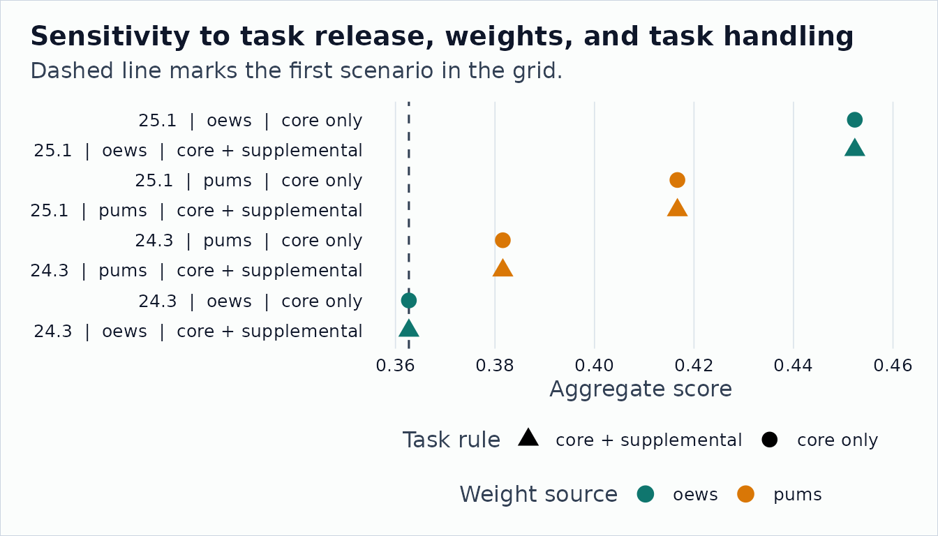

Inspect Provenance

onet_provenance(sensitivity) |>
  select(any_of(c("weight_source", "weight_year", "bridge", "measure_id"))) |>
  head(8) |>
  onet_kable()

weight_source	weight_year	measure_id
OEWS	2024	stylized_exposure
PUMS	2022	stylized_exposure
OEWS	2024	stylized_exposure
PUMS	2022	stylized_exposure
OEWS	2024	stylized_exposure
PUMS	2022	stylized_exposure
OEWS	2024	stylized_exposure
PUMS	2022	stylized_exposure

If the sign, rank, or interpretation of a result depends on one plumbing choice, say so in the write-up. Running the grid does not make a result more trustworthy; it just shows where that result is fragile.