onet2r helps you move from occupation search to
analysis-ready O*NET tables, archived O*NET releases, and BLS OEWS wage
and employment context. Current O*NET Web Services calls require a free
API key from the O*NET developer
portal. Store it in .Renviron as
ONET_API_KEY=your-api-key-here so scripts do not contain
secrets.
The live Web Services examples are opt-in for package builds because
CRAN and CI should not depend on an external API. Everything else in
this article uses local files through actual onet2r
functions.
tibble::tibble(
  setting = c("ONET_API_KEY configured", "live vignette API calls enabled"),
  value = c(has_onet_key, run_live)
) |>
onet_kable()| setting | value |
|---|---|
| ONET_API_KEY configured | FALSE |
| live vignette API calls enabled | FALSE |
Search the Current O*NET API
When live calls are enabled, the first step is usually
onet_search(), followed by a detail endpoint such as
onet_skills() or onet_abilities().
if (run_live) {
  onet_search("software developer", start = 1, end = 5) |>
    onet_kable()
} else {
  tibble::tibble(
    live_api_example = "skipped",
    reason = "Set ONET_API_KEY and ONET2R_RUN_LIVE_VIGNETTES=true to run onet_search()."
  ) |>
    onet_kable()
}| live_api_example | reason |
|---|---|
| skipped | Set ONET_API_KEY and ONET2R_RUN_LIVE_VIGNETTES=true to run onet_search(). |
if (run_live) {
  onet_skills("15-1252.00", start = 1, end = 5) |>
    onet_kable()
} else {
  tibble::tibble(
    live_api_example = "skipped",
    reason = "Set ONET_API_KEY and ONET2R_RUN_LIVE_VIGNETTES=true to run onet_skills()."
  ) |>
    onet_kable()
}| live_api_example | reason |
|---|---|
| skipped | Set ONET_API_KEY and ONET2R_RUN_LIVE_VIGNETTES=true to run onet_skills(). |
Read an Archived O*NET Table
The Web Services API serves the current release. Historical work uses
the downloadable archive tables. onet_archive_read()
normalizes those archive files into tibbles with stable columns.
abilities <- onet_archive_read(
  "30.3",
  "Abilities",
  path = archive_303,
  release_date = "2026-05-01"
)

abilities |>
  select(
    release_version,
    onet_soc_code,
    soc_code,
    element_id,
    element_name,
    data_value,
    source_date,
    domain_source
  ) |>
  head(8) |>
onet_kable()| release_version | onet_soc_code | soc_code | element_id | element_name | data_value | source_date | domain_source |
|---|---|---|---|---|---|---|---|
| 30.3 | 15-1252.00 | 15-1252 | 1.A.1.a.1 | Oral Comprehension | 4.35 | 2025-07-01 | Analyst |
| 30.3 | 15-1252.00 | 15-1252 | 1.A.1.b.1 | Problem Sensitivity | 4.50 | 2024-07-01 | Analyst |
| 30.3 | 29-1141.00 | 29-1141 | 1.A.1.a.1 | Oral Comprehension | 4.71 | 2025-08-01 | Incumbent |
| 30.3 | 29-1141.00 | 29-1141 | 1.A.1.b.1 | Problem Sensitivity | 4.90 | 2024-08-01 | Incumbent |
| 30.3 | 11-1011.00 | 11-1011 | 1.A.1.a.1 | Oral Comprehension | 4.50 | 2025-07-01 | Incumbent |
| 30.3 | 11-1011.00 | 11-1011 | 1.A.1.b.1 | Problem Sensitivity | 4.22 | 2024-07-01 | Analyst |
| 30.3 | 41-1011.00 | 41-1011 | 1.A.1.a.1 | Oral Comprehension | 4.15 | 2025-06-01 | Analyst |
Add Labor-Market Context
BLS OEWS estimates add employment and wage scale to O*NET occupation rows. The modern weighting path creates an explicit reference-SOC weight panel.
oews <- onet_oews_national(2024, path = sample_oews)
weights <- onet_weight_panel_oews(oews, year = 2024)

weights |>
onet_kable()| reference_soc_code | year | employment | weight_share | source | source_taxonomy | reference_taxonomy |
|---|---|---|---|---|---|---|
| 11-1011 | 2024 | 211230 | 0.040 | OEWS | 2018 SOC | 2018 SOC |
| 15-1252 | 2024 | 1847900 | 0.353 | OEWS | 2018 SOC | 2018 SOC |
| 29-1141 | 2024 | 3175400 | 0.607 | OEWS | 2018 SOC | 2018 SOC |
To answer a concrete question, take one ability, treat the O*NET values as the user-supplied occupation score, and aggregate with OEWS employment.
oral_scores <- abilities |>
  filter(element_id == "1.A.1.a.1") |>
  transmute(onet_soc_code, measure_score = data_value)

oral_aggregate <- onet_measure_aggregate(
  oral_scores,
  weights,
  measure_id = "oral_comprehension_fixture"
)

oral_aggregate |>
  select(-coverage, -provenance) |>
onet_kable()| measure_id | aggregate | total_employment | covered_employment | employment_coverage_share | n_occupations | n_reference_soc |
|---|---|---|---|---|---|---|
| oral_comprehension_fixture | 4.574 | 5234530 | 5234530 | 1 | 4 | 4 |
onet_provenance(oral_aggregate) |>
onet_kable()| measure_id | weight_source | weight_year | source_taxonomy | reference_taxonomy | bridge_used | crosswalk_path |
|---|---|---|---|---|---|---|
| oral_comprehension_fixture | OEWS | 2024 | 2018 SOC | 2018 SOC | FALSE | 2018 SOC -> 2018 SOC |
Compare Two Archive Releases
For historical analysis, build a panel, reconcile adjacent releases, and inspect comparability flags before interpreting changes.
panel <- onet_panel(
  "Abilities",
  versions = c("30.2", "30.3"),
  scale = "IM",
  archives = c(`30.2` = archive_302, `30.3` = archive_303),
  release_dates = c(`30.2` = "2026-02-01", `30.3` = "2026-05-01")
)

changes <- onet_panel_reconcile(
  panel,
  bridge = onet_crosswalk_bridge("2019", "2019")
)

changes |>
  select(
    to_soc_code,
    element_name,
    from_value,
    to_value,
    value_change,
    change_type,
    safely_comparable
  ) |>
  arrange(desc(abs(value_change))) |>
  head(8) |>
onet_kable()| to_soc_code | element_name | from_value | to_value | value_change | change_type | safely_comparable |
|---|---|---|---|---|---|---|
| 29-1141 | Problem Sensitivity | 4.60 | 4.90 | 0.30 | recode_or_recalc_flag | FALSE |
| 15-1252 | Oral Comprehension | 4.12 | 4.35 | 0.23 | real_update | TRUE |
| 41-1011 | Oral Comprehension | 4.00 | 4.15 | 0.15 | real_update | TRUE |
| 11-1011 | Oral Comprehension | 4.38 | 4.50 | 0.12 | real_update | FALSE |
| 15-1252 | Problem Sensitivity | 4.50 | 4.50 | 0.00 | stale_carryforward | TRUE |
| 29-1141 | Oral Comprehension | 4.71 | 4.71 | 0.00 | resampled_stable | TRUE |
| 11-1011 | Problem Sensitivity | 4.22 | 4.22 | 0.00 | stale_carryforward | TRUE |
plot_data <- changes |>
  count(change_type, name = "rows") |>
  arrange(desc(rows))

ggplot2::ggplot(plot_data, ggplot2::aes(
  x = stats::reorder(change_type, rows),
  y = rows,
  fill = change_type
)) +
  ggplot2::geom_col(width = 0.65, show.legend = FALSE) +
  ggplot2::coord_flip() +
  onet2r_discrete_fill() +
  ggplot2::labs(
    title = "What Kind of Change Was Observed?",
    subtitle = "Interpret the classification before the numeric change.",
    x = NULL,
    y = "Rows"
  ) +
  onet2r_theme()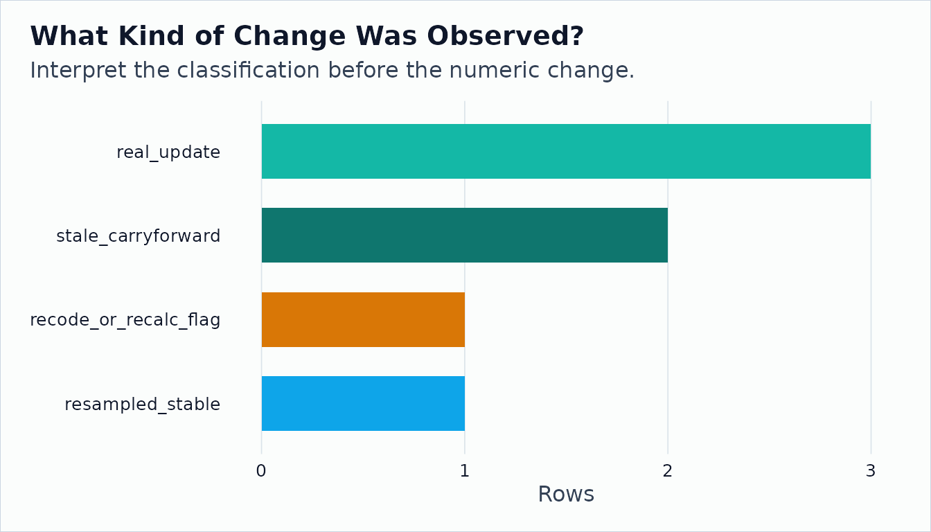
Next Steps
- Read
vignette("longitudinal-onet-background", package = "onet2r")before interpreting cross-release changes. - Read
vignette("longitudinal-archives", package = "onet2r")to assemble and reconcile archive panels. - Read
vignette("oews-wage-context", package = "onet2r")to choose and apply employment weights. - Read
vignette("stress-testing-exposure-measure", package = "onet2r")to stress test a user-supplied measure.